etf <- etf_vix[1:55, 1:3]
# Split-------------------------------
h <- 5
etf_eval <- divide_ts(etf, h)
etf_train <- etf_eval$train
etf_test <- etf_eval$test
Models with Stochastic Volatilities
By specifying cov_spec = set_sv(),
var_bayes() and vhar_bayes() fits VAR-SV and
VHAR-SV with shrinkage priors, respectively.
- Three different prior for innovation covariance, and specify through
coef_spec- Minneosta prior
- BVAR:
set_bvar() - BVHAR:
set_bvhar()andset_weight_bvhar()
- BVAR:
- SSVS prior:
set_ssvs() - Horseshoe prior:
set_horseshoe() - NG prior:
set_ng() - DL prior:
set_dl()
- Minneosta prior
-
sv_spec: prior settings for SV,set_sv() -
intercept: prior for constant term,set_intercept()
set_sv()
#> Model Specification for SV with Cholesky Prior
#>
#> Parameters: Contemporaneous coefficients, State variance, Initial state
#> Prior: Cholesky
#> ========================================================
#> Setting for 'shape':
#> [1]  rep(3, dim)
#>
#> Setting for 'scale':
#> [1]  rep(0.01, dim)
#>
#> Setting for 'initial_mean':
#> [1]  rep(1, dim)
#>
#> Setting for 'initial_prec':
#> [1]  0.1 * diag(dim)
SSVS
(fit_ssvs <- vhar_bayes(etf_train, num_chains = 2, num_iter = 20, coef_spec = set_ssvs(), cov_spec = set_sv(), include_mean = FALSE, minnesota = "longrun"))
#> Call:
#> vhar_bayes(y = etf_train, num_chains = 2, num_iter = 20, coef_spec = set_ssvs(),
#>     cov_spec = set_sv(), include_mean = FALSE, minnesota = "longrun")
#>
#> BVHAR with Stochastic Volatility
#> Fitted by Gibbs sampling
#> Number of chains: 2
#> Total number of iteration: 20
#> Number of burn-in: 10
#> ====================================================
#>
#> Parameter Record:
#> # A draws_df: 10 iterations, 2 chains, and 210 variables
#>      phi[1]   phi[2]   phi[3]  phi[4]    phi[5]    phi[6]  phi[7]    phi[8]
#> 1    0.8983  -0.0599   0.0916  -1.865  -0.08285  -0.65925  -0.223   1.60857
#> 2    0.1141   0.4634  -0.0177  -0.455  -0.02866  -0.70327   0.301   1.19827
#> 3    0.4094   0.1782  -0.0727   0.293  -0.08276   0.14471  -2.338  -0.01015
#> 4   -0.7451  -0.1365  -0.0405   0.230   0.30052  -0.39210  -0.431  -0.00581
#> 5   -0.3590   0.1685  -0.0122   0.556   0.13990  -0.09000  -0.308   0.14631
#> 6    0.4698  -0.3892   0.0172  -0.449   0.10019  -0.23203   0.387   0.08415
#> 7   -0.0563  -0.0740   0.0171   0.375   0.20512   0.00926   0.053   0.32945
#> 8    0.0203   0.0580  -0.0556   0.453   0.36827  -0.09601   0.103   0.04103
#> 9   -0.0478   0.0260  -0.0415   0.386  -0.01221  -0.17503   0.219  -0.00532
#> 10   0.0488   0.0445  -0.0428   0.024   0.00395  -0.06741   0.288   0.20163
#> # ... with 10 more draws, and 202 more variables
#> # ... hidden reserved variables {'.chain', '.iteration', '.draw'}
Horseshoe
(fit_hs <- vhar_bayes(etf_train, num_chains = 2, num_iter = 20, coef_spec = set_horseshoe(), cov_spec = set_sv(), include_mean = FALSE, minnesota = "longrun"))
#> Call:
#> vhar_bayes(y = etf_train, num_chains = 2, num_iter = 20, coef_spec = set_horseshoe(),
#>     cov_spec = set_sv(), include_mean = FALSE, minnesota = "longrun")
#>
#> BVHAR with Stochastic Volatility
#> Fitted by Gibbs sampling
#> Number of chains: 2
#> Total number of iteration: 20
#> Number of burn-in: 10
#> ====================================================
#>
#> Parameter Record:
#> # A draws_df: 10 iterations, 2 chains, and 215 variables
#>      phi[1]   phi[2]   phi[3]   phi[4]     phi[5]    phi[6]   phi[7]   phi[8]
#> 1    0.2362   0.1463  -0.0517  -0.0742  -1.66e-03  -0.06187   0.1833   0.1611
#> 2    0.1831   0.1819  -0.1090   0.1610   8.89e-03  -0.00887   0.0232   0.1321
#> 3    0.2455   0.1286  -0.0703   0.1222  -8.73e-03  -0.05949  -0.1382   0.1039
#> 4    0.0963   0.1087  -0.1558   0.1166   5.65e-03   0.02191   0.1070   0.1130
#> 5    0.0372   0.1497  -0.1538   0.1946  -2.67e-03  -0.02359  -0.0237   0.2995
#> 6   -0.0573   0.1079  -0.2566   0.5879   7.73e-04   0.01944   0.0156   0.0960
#> 7    0.1053   0.0943  -0.1837   0.2004   1.80e-03   0.10304   0.0697   0.2996
#> 8    0.0232  -0.0412  -0.1501   0.3045  -2.18e-04  -0.13582   0.0191  -0.0158
#> 9    0.0504   0.1025  -0.1617   0.2406   9.16e-05   0.00157  -0.0346   0.2380
#> 10   0.0223   0.0831  -0.1558   0.1374  -1.42e-04  -0.01194   0.0992   0.1018
#> # ... with 10 more draws, and 207 more variables
#> # ... hidden reserved variables {'.chain', '.iteration', '.draw'}
Normal-Gamma prior
(fit_ng <- vhar_bayes(etf_train, num_chains = 2, num_iter = 20, coef_spec = set_ng(), cov_spec = set_sv(), include_mean = FALSE, minnesota = "longrun"))
#> Call:
#> vhar_bayes(y = etf_train, num_chains = 2, num_iter = 20, coef_spec = set_ng(),
#>     cov_spec = set_sv(), include_mean = FALSE, minnesota = "longrun")
#>
#> BVHAR with Stochastic Volatility
#> Fitted by Metropolis-within-Gibbs
#> Number of chains: 2
#> Total number of iteration: 20
#> Number of burn-in: 10
#> ====================================================
#>
#> Parameter Record:
#> # A draws_df: 10 iterations, 2 chains, and 188 variables
#>       phi[1]    phi[2]    phi[3]   phi[4]   phi[5]    phi[6]   phi[7]  phi[8]
#> 1   -0.12129   0.46645   0.00633  -0.2542   0.0983  -0.12326   0.8472   1.195
#> 2   -0.06070  -0.03576   0.26003   0.3627  -0.0493   0.10581  -0.6588  -0.233
#> 3   -0.12030   0.09924   0.06952   0.6217   0.2413   0.20229  -0.3341   0.896
#> 4   -0.05398  -0.83427   0.32929  -0.7151   0.5682  -0.77103   1.8176   0.311
#> 5   -0.08097  -0.00470  -0.01688   1.0261  -0.0247   0.20555  -0.7039   0.113
#> 6   -0.09683   0.00503   0.00561   0.9218  -0.3035  -0.02819  -0.8611   0.264
#> 7   -0.04152   0.00752  -0.03170   0.8207   0.4101  -0.07181   0.0765   0.490
#> 8    0.00444  -0.18934   0.07036   0.4606   0.3786   0.07076   0.0405   0.923
#> 9   -0.00374   0.07720  -0.05009  -0.0199  -0.1694   0.08192  -0.0237   1.378
#> 10  -0.04211  -0.07598   0.11729  -0.0914   0.0158   0.00741  -0.0348   1.455
#> # ... with 10 more draws, and 180 more variables
#> # ... hidden reserved variables {'.chain', '.iteration', '.draw'}
Dirichlet-Laplace prior
(fit_dl <- vhar_bayes(etf_train, num_chains = 2, num_iter = 20, coef_spec = set_dl(), cov_spec = set_sv(), include_mean = FALSE, minnesota = "longrun"))
#> Call:
#> vhar_bayes(y = etf_train, num_chains = 2, num_iter = 20, coef_spec = set_dl(),
#>     cov_spec = set_sv(), include_mean = FALSE, minnesota = "longrun")
#>
#> BVHAR with Stochastic Volatility
#> Fitted by Gibbs sampling
#> Number of chains: 2
#> Total number of iteration: 20
#> Number of burn-in: 10
#> ====================================================
#>
#> Parameter Record:
#> # A draws_df: 10 iterations, 2 chains, and 182 variables
#>       phi[1]    phi[2]     phi[3]    phi[4]    phi[5]    phi[6]   phi[7]
#> 1    0.16969  -0.24454  -0.126475  -0.06212  -0.00613   0.10133   0.2047
#> 2    0.13486  -0.04642  -0.148850   0.29445  -0.00510   0.03525   0.1231
#> 3    0.09879  -0.00417   0.012937   0.08343  -0.00992  -0.03586   0.0190
#> 4   -0.05609  -0.02515  -0.009510   0.27036  -0.04458  -0.00890  -0.0160
#> 5    0.00416   0.02970   0.007852  -0.08386  -0.01198  -0.13536   0.0647
#> 6   -0.00753  -0.13360  -0.053984   0.06215   0.01830   0.02951  -0.1006
#> 7    0.03670   0.06412  -0.129178  -0.00837   0.00700   0.06118   0.1877
#> 8    0.04795   0.01647  -0.091950   0.01753   0.02061   0.03345   0.4122
#> 9    0.00318   0.01126   0.000964   0.01404  -0.00825  -0.01743   0.3645
#> 10   0.04623  -0.09924   0.000799  -0.00658   0.02443   0.00132   0.3980
#>        phi[8]
#> 1    8.58e-05
#> 2   -8.17e-04
#> 3   -7.97e-04
#> 4    2.09e-03
#> 5    5.46e-03
#> 6    1.57e-02
#> 7    3.77e-01
#> 8    5.26e-01
#> 9    4.34e-01
#> 10   3.80e-01
#> # ... with 10 more draws, and 174 more variables
#> # ... hidden reserved variables {'.chain', '.iteration', '.draw'}
Bayesian visualization
autoplot() also provides Bayesian visualization.
type = "trace" gives MCMC trace plot.
autoplot(fit_hs, type = "trace", regex_pars = "tau")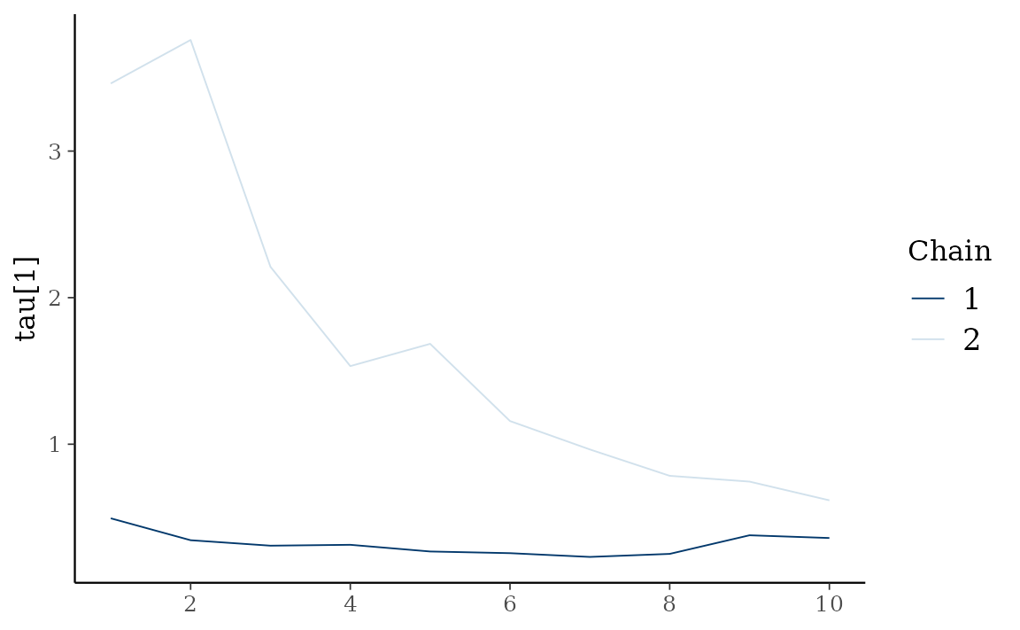
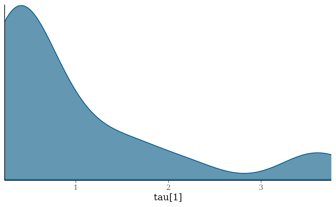
type = "dens" draws MCMC density plot.
autoplot(fit_hs, type = "dens", regex_pars = "tau")